Working with fMRI data using R

Overview

Teaching: 10 min
Exercises: 10 min

Questions

• What is fMRI?

• How can I read fMRI data in R?

• How can I visualise fMRI data with R?

Objectives

• Have a basic understanding of where the data comes from.

Recap: what is fMRI?

MRI is an imaging technique, with which we can take scans of muscles, bones, brains,… fMRI is when we repeatedly take MRI scans of the brain. This allows us to see the brain in action when it’s performing tasks or in rest etc.

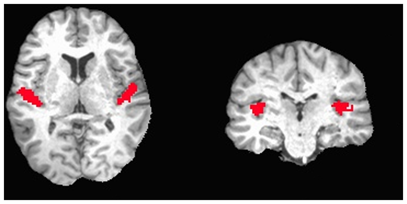
Imagine a subject listening to broadband noise for 15 seconds, and then listening to silence for 15 seconds, and repeat this for 10 times while taking brain scans every 3 seconds. Afterwards, we can compare the scans during silence with the scans during music, and end up with an image like the following from Okada et al., 2013. The brain image in the back is a structural MRI, the red blobs are the parts of the brain that show a significant difference between the two conditions.

In reality, the analysis of the data is much more complex than ‘comparing images from two conditions’ and there exist thousands of ways to analyse the data. During this lesson, we will touch a few very basic methods, but a more thorough discussion is outside the scope. We will assume that all the data is preprocessed, which means that:

• the data are corrected for motion
• the data are corrected for distortions
• the data from different subjects are aligned to a common template
• …

Reading and visualising fMRI data with R/neuroconductor.

After opening RStudio, we want to set our working directory to the directory we created during set up, where we can find the data:

setwd("~/Desktop/validating-fmri/data")

Neuroconductor is an open-source platform for analysing neuroimaging (and other) data. It hosts multiple packages to analyse data using different software. We will mostly use its base library neurobase. To install, run:

source("https://neuroconductor.org/neurocLite.R")
neuro_install("neurobase", release = "stable")

The data is located in the directory data in the working directory. Now we can load the data into R using the function readnii.

library(neurobase)
data <- readnii("sub-10159/sub-10159_task-rest_bold_space-MNI152NLin2009cAsym_preproc.nii.gz")

The function readnii requires one argument: the name of the file we want to read. This needs to be character string, which is why we put it in quotes. We saved the data to the variable sub70083. What comes out is an object of type oro.nifti. Essentially, it is a 4D array, with extra metadata specific to fMRI data. We can therefore apply functions that we can apply to arrays. Let’s look for example at the shape of our data.

dim(data)

[1]  65  77  49 152

This shows us that the first three dimensions are 65 x 77 x 49. These correspond to the x-, y- and z-coordinates of the brain. The fourth dimension is time, which means there are 152 time points measured.

We can also run a function from neurobase that only works on this type of object:

check_nifti(data)

NIfTI-1 format
  Type            : nifti
  Data Type       : 16 (FLOAT32)
  Bits per Pixel  : 32
  Slice Code      : 0 (Unknown)
  Intent Code     : 0 (None)
  Qform Code      : 2 (Aligned_Anat)
  Sform Code      : 1 (Scanner_Anat)
  Dimension       : 65 x 77 x 49 x 152
  Pixel Dimension : 3 x 3 x 4 x 2
  Voxel Units     : Unknown
  Time Units      : sec

This shows some information that is stored in the “header” of the file. For example, it tells us the pixel dimensions. The first three numbers tell us the size of the voxels in space: 3 x 3 x 4 cm. The last number tells us the dimension in time: a scan was taken every 2 seconds.

Another interesting function is the visualisation of nifti’s. Note that we only visualise one timepoint, the first one. R will automatically show the first timepoint.

orthographic(data)

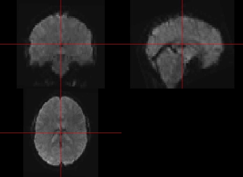
If you’re not sure about how to use a certain function, you can call for help:

?orthographic

You will see that there are many more arguments that can be passed to the function orthographic. For example the argument xyz allows us to specify where to draw the cross-hairs. Let’s try the following:

orthographic(data,xyz=c(20,20,30))

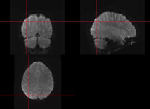
To look at the value of one specific point in time and space, we can use indexes. Remember our cross-hair in the figure was at the first timepoint at coordinates (20,20,30).
The following example shows the exact value of this point in the figure at the first timepoint.

data[20,20,30,1]

[1] 1148.524

This shows that the value at the coordinates (20,20,30) at the first timepoint in the matrix os 1000.697. The units of the data are a derivative of how much oxygen is in the blood, so in itself pretty meaningless. Especially when you know that during preprocessing, the average is set to 1000. What is more interesting is to look at how the value changes over time, which we can do by omitting the index in the 4th dimension:

data[20,20,30,]

[1] 1148.524 1148.461 1142.563 1141.060 1127.099 1131.675 1135.632 1128.941
  [9] 1160.061 1161.512 1137.481 1116.822 1109.309 1109.323 1093.169 1110.955
 [17] 1109.561 1116.910 1134.975 1118.357 1132.719 1150.193 1165.766 1173.594
 [25] 1176.839 1142.286 1145.902 1159.892 1152.587 1136.450 1127.974 1148.936
 [33] 1152.663 1174.247 1168.272 1147.255 1159.906 1184.832 1145.608 1141.148
 [41] 1132.086 1137.863 1133.563 1143.711 1141.173 1128.889 1124.897 1132.619
 [49] 1144.724 1153.767 1133.262 1135.230 1137.793 1165.782 1160.442 1159.418
 [57] 1165.768 1156.091 1169.558 1182.266 1167.106 1157.483 1163.735 1131.992
 [65] 1121.514 1111.989 1121.143 1141.684 1122.967 1126.063 1121.025 1138.645
 [73] 1132.201 1133.171 1132.688 1134.140 1127.046 1127.342 1134.374 1148.151
 [81] 1147.634 1145.883 1143.286 1142.210 1138.209 1123.161 1148.567 1149.430
 [89] 1155.253 1115.818 1116.521 1119.263 1136.349 1144.674 1151.027 1158.472
 [97] 1145.075 1124.284 1120.904 1129.625 1131.517 1120.666 1126.623 1109.636
[105] 1093.798 1126.940 1126.045 1120.136 1133.749 1101.970 1098.026 1116.716
[113] 1142.895 1143.010 1138.357 1127.057 1102.292 1122.499 1136.995 1126.363
[121] 1137.567 1122.647 1142.551 1131.645 1125.780 1120.023 1122.369 1132.125
[129] 1104.158 1107.103 1088.539 1116.694 1149.974 1146.161 1140.482 1114.848
[137] 1099.089 1121.268 1141.496 1141.877 1129.998 1106.165 1107.426 1105.125
[145] 1089.509 1103.882 1114.204 1113.552 1096.908 1104.983 1102.881 1121.604

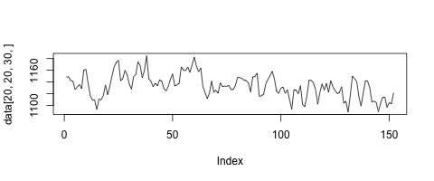
If we plot this vector, we can see how the measured signal in this voxel changes over time.

plot(data[20,20,30,],type='l')

Exercises

Now that we know how to read, inspect and visualise fMRI data, it’s time for some exercises ! In the data-folder, there is for each subject 3 nifti-images:

• mask: sub-XXXXX_task-rest_bold_space-MNI152NLin2009cAsym_brainmask.nii.gz
• rest: sub-XXXXX_task-rest_bold_space-MNI152NLin2009cAsym_preproc.nii.gz
• anatomical: sub-XXXXX_T1w_preproc.nii.gz

We have looked at the functional rest data. Now look at the anatomical scan yourself.

• Read in the anatomical data.
• What are the dimensions of the anatomical data? Compare with the dimensions of the rest scan.
• Visualise the data.
• Set the color of the cross-hairs to blue
• Look at what the function double_ortho does, and use it to plot the rest scan (the first timepoint) and the anatomical scan.

Key Points

• fMRI data is a time series of 3D images of the brain.

• Visualising and manipulating fMRI nifti images can be done with neurobase.