Using real data to validate task fMRI.
Overview
Teaching: 20 min
Exercises: 20 minQuestions
What’s with that Eklund paper?
How do we usually assess whether a part in the brain is active during task fMRI?
How do we create a random regressor?
Objectives
Understand how Eklund defines the null hypothesis for fMRI.
Do a simulation that is somewhat similar to what Eklund did, on the parcel level.
The Eklund paper
Last year, Anders Eklund published a paper validating cluster inference. He found that the false positive rate is much higher than the nominal level. His really cool approach was to ‘pretend’ the resting state data is in fact coming from a task experiment with a random design matrix. Given that the participants (and the experimentors) were unaware of the task, the null hypothesis should be true.
Loading the necessary libraries
library(neuRosim)
Let’s try that as well !
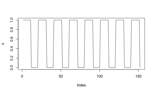
Assume we are designing an fMRI experiment, with a blocked design (10 seconds on / 10 seconds off). We can use neuRosim to create our design.
totaltime <- 152*2
onsets <- seq(1,totaltime,40)
dur <- 20
s <- specifydesign(totaltime=totaltime,onsets=list(onsets),durations=dur,
                   accuracy=1,effectsize=1,TR=2)
plot(s,type='l')
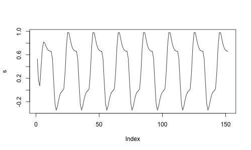
We could probably expect neurons to be firing very fast, but the signal that we measure is a dependent of the oxygen in the blood which comes only a few seconds later. The signal that we expect looks like this:
s <- specifydesign(totaltime=totaltime,onsets=list(onsets),durations=dur,
                   accuracy=1,effectsize=1,TR=2,conv="double-gamma")
plot(s,type='l')
If we would now estimate whether a voxel is significantly related to the task, we would regress the signal from a resting state dataset onto this design matrix. If we do that, we can assume the null hypothesis: any relation between the design and the signal is by chance.
Ideally, we would now do this for all voxels, but for computational reasons, we’ll focus on parcels (1000’s of voxels vs 39 parcels).
Ideally, we would now extract the time series ourselves, but of or computational reasons, the time series are already extracted in the data folder (CNP_ts/).
Let’s look at one subject.
datdir <- 'CNP_ts/'
files <- list.files(datdir)
timeseries <- read.table(paste0(datdir,files[2]),sep=",")
head(timeseries,2)
V1        V2        V3         V4        V5        V6         V7
1 -0.1950061 0.2783514 -0.559840 -0.3996359 1.0245059 1.0665180  0.1788859

2 -0.5303118 0.1370437 -0.731119 -0.5694947 0.7857156 0.4777555 -0.1150351
V8         V9      V10      V11       V12      V13      V14       V15
1 0.6270506  0.1775939 1.417099 1.261883 0.7566771 2.252137 1.569789 1.3837699
2 0.1530690 -0.3995555 1.136001 1.172791 0.3141784 1.583866 1.139964 0.9155217
V16        V17        V18        V19       V20        V21        V22
1 1.318610  0.3197243 -0.3064194 -0.4392510 -0.898600 -0.4151906 -0.3008893
2 1.027048 -0.6107545 -0.6941234 -0.8259567 -1.006105 -0.4625272 -0.4666169
 V23       V24       V25        V26        V27        V28       V29
1 1.0183324243 1.1613632 1.1515451  0.3756378  0.1103843  0.1391557 0.3727925
2 0.0007187072 0.8576137 0.5978735 -0.3542256 -0.5289335 -0.1650633 0.0348114
V30       V31      V32        V33        V34         V35       V36
1 0.831866 -1.354775 1.777831 0.07237729 -0.3987264 -0.03841347 -1.038179
2 0.247771 -1.256893 1.514126 0.04430596 -0.8933236 -0.27476992 -1.729911
V37        V38        V39
1 1.2687749 -0.2517349 -0.6559813
2 0.9014437 -0.7673380 -0.9268040
plot(timeseries$V1,type="l")
lines(s,col=2)
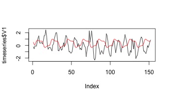
Now let’s regress our data onto a random design.
timeseries$design <- s
model <- lm("V1 ~ design",data=timeseries)
summary(model)
Call:
lm(formula = "V1 ~ design", data = timeseries)


Residuals:
     Min       1Q   Median       3Q      Max
-2.48198 -0.73232 -0.02282  0.74389  2.37832

Coefficients:
            Estimate Std. Error t value Pr(>|t|)
(Intercept)   0.1417     0.1049   1.351   0.1788
design       -0.3898     0.1851  -2.106   0.0369 *
---
Signif. codes:  0 ‘***’ 0.001 ‘**’ 0.01 ‘*’ 0.05 ‘.’ 0.1 ‘ ’ 1

Residual standard error: 0.9921 on 150 degrees of freedom
Multiple R-squared:  0.02871,   Adjusted R-squared:  0.02224
F-statistic: 4.434 on 1 and 150 DF,  p-value: 0.03689
summary(model)$coefficients
Estimate Std. Error   t value   Pr(>|t|)
(Intercept)  0.1416964  0.1048957  1.350832 0.17878356
design      -0.3898186  0.1851187 -2.105777 0.03688945
pval <- summary(model)$coefficients[2,4]
tval <- summary(model)$coefficients[2,3]
print(paste("pvalue: ",pval," - tvalue:",tval))
[1] "pvalue: 0.0368894469806956 - tvalue: -2.10577655168616"
Now we can loop this.
pvals <- c()
tvals <- c()
i = 1
for (file in files){
  timeseries <- read.table(paste0(datdir,file),sep=",")
  timeseries$design <- s
  model <- lm("V1 ~ design",data=timeseries)
  pvals[i] <- summary(model)$coefficients[2,4]
  tvals[i] <- summary(model)$coefficients[2,3]
  i = i+1
}

sum(pvals<0.05)/length(pvals)
[1] 0.2192308
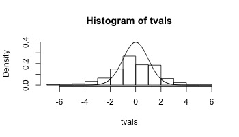
Let’s look at the distribution of t-values.
hist(tvals,freq=FALSE,ylim=c(0,0.4))
x <- seq(-6,6,length=1000)
y <- dt(x,151)
lines(x,y)
Exercises
- What happens when you choose a more random design (onsets not evenly spaced)?
- Do you observe the same pattern in another?
Can you make a loop (around the loop) that saves the false positive rate for all parcels.
hint: with
paste0("V",j,"~design"), you can make the model specification dependent on an index j.
Key Points
It can be very insightful to use resting data to validate task methods.